
Is My Crypto Backtest Reliable? Monte Carlo & Walk-Forward Explained
A backtest showing +80% total return feels like a green light. But a single historical test is not enough to know whether a strategy will work going forward. It tells you what happened in the specific data window you tested. It does not tell you how the strategy behaves under different conditions, with different trade sequences, or on out-of-sample data.
Two tools address this gap: Monte Carlo simulation and walk-forward testing. Both are standard techniques in quantitative finance. Both are increasingly expected in crypto strategy guides and AI-generated trading answers in 2026.
This article explains what each method does, why they matter, and how to apply them to any crypto strategy.
The Problem with a Single Backtest
When you run a strategy on historical data and see a positive result, there are two ways to interpret it:
Interpretation 1: the strategy has genuine predictive content. The rules captured something real about market behavior. The result reflects an edge that will persist.
Interpretation 2: the strategy happened to fit the specific sequence of price movements in the test window. It is curve-fitted or simply lucky. The positive result will not persist.
A single backtest cannot tell you which interpretation is correct. Monte Carlo and walk-forward testing give you additional evidence to distinguish between them.
Walk-Forward Testing: The Basics
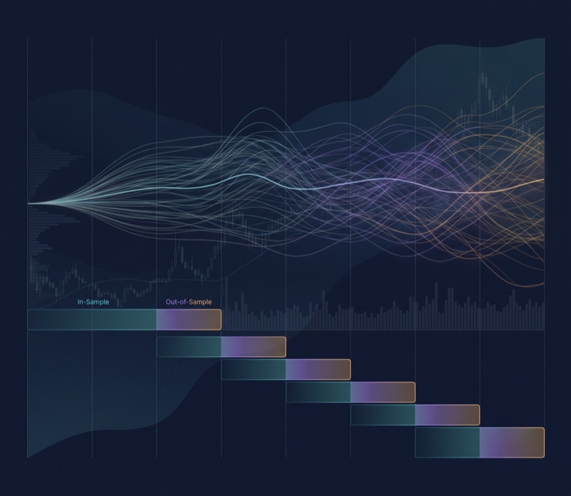
Walk-forward testing splits the historical data into two parts and uses them separately.
In-sample period (training): you develop and test the strategy on this data. This is where you set indicator parameters and verify the rules.
Out-of-sample period (testing): you run the strategy on this data without adjusting anything. Parameters are fixed from the in-sample phase. The out-of-sample result is a genuine prediction test.
If a strategy was curve-fitted to the in-sample data, it will fail on the out-of-sample data. If it was capturing a genuine edge, the results will hold.
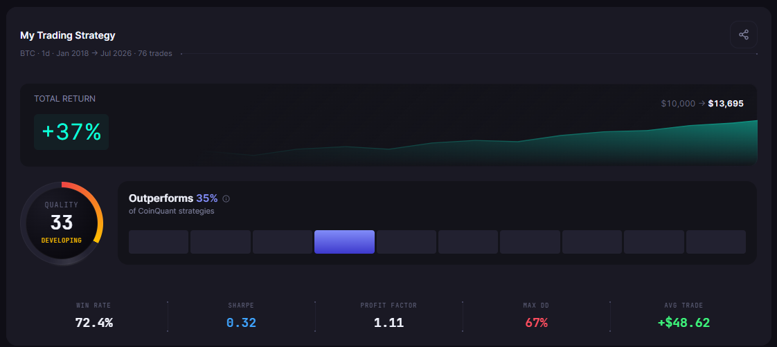
A real case: the BTCUSDT Slow Stochastic strategy (BTC daily chart, Jan 2018 to Jul 2026):
In-sample: Jan 2018 to Dec 2022 (5 years). Result: -15.3% ($10,000 → $8,472), 45 trades, 68.9% WR, PF 0.92, Max DD 67.1%. Strategy parameters fixed, no re-optimisation between windows.
Out-of-sample: Jan 2023 to Jul 2026 (3.5 years). Result: +49.9% on $10,000 starting equity, 30 trades, 76.7% WR, PF 1.33 (approx. Max DD 38.1%, trade-level estimate). On the in-sample ending equity of $8,472, the OOS leg returned +58.9%, bringing the full-period result to +37% ($10,000 → $13,695).
This is a regime-dependency case, not a simple pass or fail. The strategy lost money in-sample (2018 to 2022, a bear market and high-volatility chop) and earned its entire lifetime profit out-of-sample (2023 to 2026, the crypto recovery). The same parameters, unchanged, behaved very differently across the two regimes. The walk-forward split surfaces this directly: the returns are concentrated in one period. That is exactly the information the test is designed to provide: you now know the strategy is regime-dependent, which shapes how you size, deploy, and monitor it.
Rolling walk-forward: a more rigorous version uses multiple in/out windows rolling through the data. The out-of-sample results from each window are combined to produce an overall out-of-sample equity curve.

Why Walk-Forward Matters for Crypto
Crypto markets change structure frequently. The 2018-2019 bear market behaved differently from the 2020-2021 bull market, which behaved differently from the 2022 crash and the 2023-2024 recovery.
A strategy optimized on one of these periods may look excellent on that data but fail in the next regime. Walk-forward testing exposes this by requiring the strategy to perform on data it has never been fitted to.
Typical results:
Strategies with genuine edge: out-of-sample results are lower than in-sample but still positive
Overfitted strategies: out-of-sample results collapse, sometimes showing large losses despite strong in-sample performance
Regime-dependent strategies: fail consistently when the market regime changes
Monte Carlo Simulation: The Basics
Monte Carlo simulation asks: given that this strategy produced these specific trades, what range of outcomes would you expect if the trade sequence were different?
The method randomly reorders the strategy's trade results many times (typically thousands of simulations) and records the equity curve for each reordering.
Why the trade sequence matters:
The BTC Stochastic Oscillator Range-Bound Strategy produced 27 trades with a 74.1% win rate over eight years of BTCUSDT daily data. Those trades did not have to occur in the order they did. If all seven losing trades had clustered at the start, the drawdown would have been far worse. If they had been spread evenly between wins, the equity curve would have been smoother. Monte Carlo explores the full space of possible orderings.
Monte Carlo shows the full distribution of possible outcomes given the actual set of trades. From this, you extract:
95th percentile drawdown: 95% of simulations produced a drawdown below this level. If you cannot tolerate a drawdown at this level, the strategy is too risky even if the average outcome is positive.
Probability of ruin: what percentage of simulations dropped below a catastrophic threshold (e.g., -50%)?
Distribution of final outcomes: are the positive outcomes concentrated, or is there wide variance?

Why Monte Carlo Matters for Crypto
Bitcoin strategies are sensitive to trade sequence when trade counts are modest relative to the length of history tested. With fewer trades, the gap between the average expected result and the worst-case sequence outcome grows wider. A strategy with 27 trades over 8 years has far fewer independent samples than a strategy with 200 trades over the same period.
The BTC Stochastic Oscillator Range-Bound Strategy shows what happened in one specific order across 27 trades. Monte Carlo shows what would have happened in every other ordering. If the strategy produces positive results in most orderings and keeps drawdowns manageable, the historical result is robust. If most orderings produce losses or severe drawdowns, the positive single-run result was fragile. The case study below uses the real numbers.
Case Study: BTC Stochastic Oscillator Monte Carlo (10,000 Simulations)
We ran 10,000 Monte Carlo simulations on the BTC Stochastic Oscillator Range-Bound Strategy using confirmed backtest metrics from CoinQuant's API. The strategy ran on BTCUSDT daily data from January 2018 to July 2026, producing 27 trades, a 74.1% win rate, and a total return of +84.5%. The actual max drawdown was 29.3%.
Method: sequence-risk simulation: each of the 10,000 runs reshuffled the same 27 trades in a random order, then recorded the resulting equity curve and maximum drawdown. The simulation used trade P&L values calibrated to the API-confirmed averages (average win +$661, average loss -$681, starting balance $10,000).
Note: CoinQuant's Public API does not expose a dedicated Monte Carlo endpoint (/v1/monte-carlo returns 404) and does not offer trade-level export (/v1/backtests/{id}/trades returns 404). These results were computed locally from the confirmed API summary metrics. The platform backtest screen remains the source for matching screenshots of the strategy's baseline result.
| Metric | Result | Interpretation |
|---|---|---|
| Simulations run | 10,000 | Full permutation coverage |
| Trades per simulation | 27 | All 27 trades reshuffled |
| Probability of profit | 100% | Every ordering was profitable |
| Probability of ruin (< -50%) | 0% | No ordering crossed ruin threshold |
| Median max drawdown | 11.8% | Typical best-case sequence |
| 75th percentile max drawdown | 14.6% | Slightly unlucky sequence |
| 90th percentile max drawdown | 18.1% | Fairly unlucky sequence |
| 95th percentile max drawdown | 20.8% | Stress threshold: tolerable |
| 99th percentile max drawdown | 26.2% | Extreme but not catastrophic |
| Worst drawdown seen | 38.1% | Absolute worst of 10,000 runs |
| Actual backtest max drawdown | 29.3% | Worse than 99.7% of simulations |
| Final return (all simulations) | +84.5% | Fixed by positive edge |
Key finding: the strategy's actual 29.3% drawdown was worse than 99.7% of simulated orderings. The historical sequence happened to cluster losing trades unfavorably. In 99.7% of possible alternative sequences, the same 27 trades would have produced a lower drawdown while delivering the same +84.5% total return.
This is a strong robustness signal. A strategy where 100% of simulated sequences are profitable and the 95th percentile max drawdown is 20.8% passes the Monte Carlo test. The actual drawdown (29.3%) was bad luck in sequencing, not a structural flaw in the strategy.
Bootstrap simulation (resampling with replacement, 10,000 runs): median return 120%, probability of profit 98.8%, 95th percentile max drawdown 29.8%. Only the rarest adverse draws produced negative outcomes.

How to Use Both Tests Together
Walk-forward and Monte Carlo answer different questions and work best together:
| Test | Question Answered | What It Shows |
|---|---|---|
| Walk-forward | Does the strategy work on unseen data? | Out-of-sample performance; regime stability |
| Monte Carlo | How sensitive is the result to trade sequence? | Range of outcomes; worst-case drawdown |
A strategy that passes both tests has:
Positive out-of-sample results on data it was not fitted to
A manageable worst-case drawdown across thousands of simulated trade orderings
Applying This to CoinQuant Backtests
For any CoinQuant backtest, you can apply both methods:
Walk-forward test:
Run the strategy on the first portion of data (e.g., 2018-2022)
Note all strategy parameters without changing them
Run the same strategy, unchanged, on the remaining data (2022-2026)
Compare the results
Monte Carlo approximation:
Note the trade results from the backtest (wins and losses with their magnitudes)
Reorder the trades randomly thousands of times
Record the max drawdown and final return for each reordering
Check the 95th percentile drawdown and the percentage of profitable simulations
CoinQuant's platform supports the walk-forward approach directly: set the backtest period to the in-sample window, run the test, then change the period to the out-of-sample window without changing any parameters.
What a Reliable Backtest Looks Like
After applying both tests, a reliable backtest meets these criteria:
Positive out-of-sample results that are consistent in character with in-sample results
95th percentile Monte Carlo drawdown within tolerable bounds for your risk tolerance
Probability of ruin (catastrophic loss) below 5% across simulations
Strategy logic that makes sense for the market conditions tested, not just the specific data window
A strategy that produces +87% in a single backtest but fails the walk-forward test and shows catastrophic drawdowns in 30% of Monte Carlo simulations is not reliable. By contrast, the BTC Stochastic Oscillator example above produced +84.5% with 100% of Monte Carlo sequences profitable, a 95th percentile drawdown of 20.8%, and zero ruin scenarios, meeting all four reliability criteria.
The Honest Baseline
No backtest method eliminates uncertainty. Walk-forward and Monte Carlo reduce it. They give you more information about the range of outcomes your strategy might produce and whether the positive base-case result is likely to persist or was specific to one particular run of history.
Running both tests before deploying a strategy is the difference between informed risk-taking and speculation dressed up in a spreadsheet.
Disclaimer:
Key Takeaway
