Ethereum has been in a consolidation range since late 2025. Grid and range-trading strategies are designed exactly for this type of environment: price oscillates within a band, and the strategy profits by buying near the bottom of the range and selling near the top repeatedly.

But the question traders should ask before deploying any grid strategy is not whether it fits the current market structure in theory. It is whether a specific implementation of that structure held up during the last six months of actual market data. This backtest runs the numbers on one concrete setup, reports the results exactly as they came out, and explains what they mean.

The Strategy: Bollinger Band Grid on Ethereum

This backtest uses Bollinger Bands (20-period, 2.0 standard deviations) as dynamic grid levels on ETHUSDT:

• The lower band acts as the buy level. When price touches it, the strategy enters long.

• The upper band acts as the sell level. When price reaches it, the strategy closes the position.

This is a long-only implementation. The strategy only buys; it does not short Ethereum when price touches the upper band. The logic is directionally biased toward range recovery: every entry assumes the price deviation from the mean is temporary and that the price will revert toward the upper band within the holding period.

Bollinger Bands recreate grid logic dynamically: the bands tighten during low volatility and widen during high volatility, automatically adjusting the effective grid range to current market conditions. This is more adaptive than fixed-level grids, which define static buy and sell zones and can become irrelevant if the asset moves outside the originally defined range.

The adaptive behaviour makes Bollinger Band grids particularly suited to assets that oscillate with varying amplitude, which describes Ethereum's 2025-2026 market structure reasonably well. The 20-period, 2.0 standard deviation setting is a conventional default, covering roughly 95% of recent price observations under the assumption of normally distributed returns.

Setup on CoinQuant

• Instrument: ETHUSDT

• Timeframe: 1-hour

• Indicator: Bollinger Bands, 20-period, 2.0 standard deviations

• Entry: price touches the lower Bollinger Band

• Exit: price reaches the upper Bollinger Band

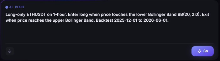
Plain-English prompt in CoinQuant: "Long-only ETHUSDT on the 1-hour chart. Enter when price touches the lower Bollinger Band (20, 2.0). Exit when price reaches the upper Bollinger Band. Backtest December 2025 to June 2026."

Backtest Results: December 2025 to June 2026

The backtest ran on the following conditions:

• 6 months of ETHUSDT 1-hour data

• Kaiko institutional data via CoinQuant, sourced directly from major exchanges

• Fees set at 0.1% per trade, applied on entry and exit

• No leverage. Initial capital $10,000

The 0.1% fee assumption reflects standard taker fees on major exchanges, a conservative but realistic input for any retail trader running this strategy.

What the Results Show

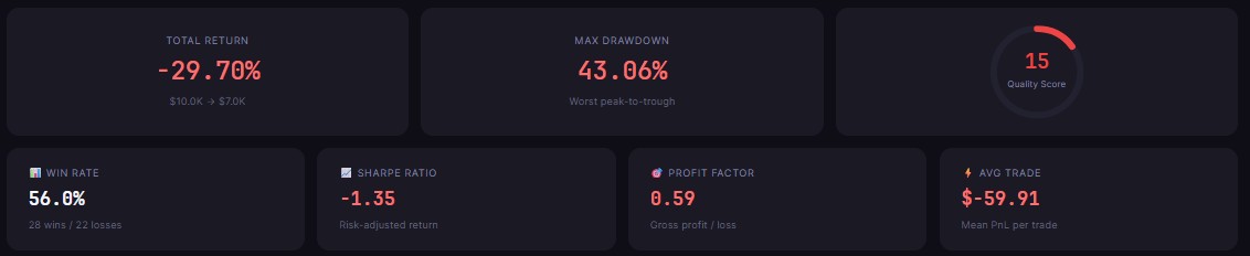
56% win rate across 50 trades confirms the range-bounce logic was correct more often than not. In 28 of 50 cases, Ethereum that touched the lower Bollinger Band recovered to the upper band before the strategy was stopped out. That is a majority: the directional assumption was right on most trades.

The problem is visible in the total return: a 56% win rate did not produce a profitable result because the losing trades were disproportionately larger than the winning ones. A strategy can be right more often than it is wrong and still lose money if the loss size on the wrong trades is large enough. This result illustrates that asymmetry directly.

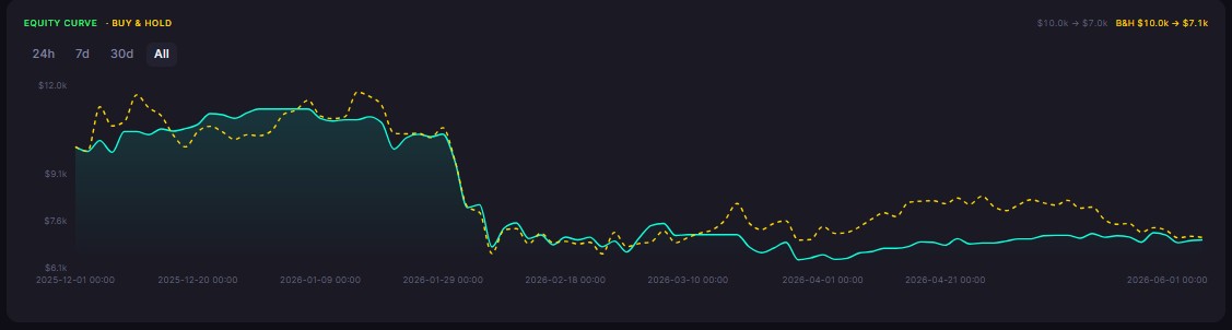
The -29.70% total return reflects the directional moves ETH made during this period: the account fell from $10,000 to $7,030. When Ethereum dropped sharply and did not immediately recover to the upper Bollinger Band, the strategy held the position through the loss.

In a genuine ranging market, this holding behaviour is correct: the price eventually reverts. But during this six-month window, ETH experienced several directional breaks, periods where the price fell through the lower band and kept moving lower, driven by macro risk-off events and protocol-specific volatility rather than normal oscillation around a stable mean. Those periods are where the drawdown accumulated.

The Sharpe Ratio of -1.35 means the strategy consistently absorbed significant volatility without generating compensating returns. For every unit of risk taken, the outcome was negative, a worse risk-adjusted result than holding cash over the same period.

A Sharpe ratio below zero does not mean the strategy was unlucky. It means the return per unit of risk was structurally negative: the volatility the strategy absorbed was not being converted into gains.

The Profit Factor of 0.59 puts the imbalance in concrete terms: for every $1.00 lost across all trades, the strategy recovered only $0.59 in gross profit. With an average trade result of -$59.91 across 50 positions, the losses compounded steadily throughout the six-month window.

These three numbers, Sharpe, Profit Factor, and average trade, collectively describe a strategy where the loss mechanics were consistently larger than the gain mechanics.

The -43.06% max drawdown is the sharpest number in the dataset. It reflects the periods when ETH broke the lower Bollinger Band and continued falling, leaving open positions deep in loss before any recovery.

A 43% drawdown means the account was down $4,306 from its peak at some point during the six months. For most traders, this would trigger a manual override of the strategy, which is precisely the kind of emotional exit that destroys the coherence of a systematic approach.

A Quality Score of 15 out of 100 captures all of these factors together: poor absolute return, large drawdown, negative risk-adjusted performance, and a profit factor well below 1.0. The score confirms this configuration is not deployable without significant parameter changes.

Key observations from the data:

• 50 trades in 6 months on the 1-hour chart means high frequency. At 0.1% per trade, fees across 50 trades compound significantly. Moving to the 4-hour timeframe would reduce trade count and fee drag.

• Win rate of 56% with a -29.70% total return confirms that winning trades were materially smaller than losing trades on average. The Profit Factor of 0.59 quantifies the exact asymmetry; losers outweighed winners by 41 cents on every dollar.

• ETH tends to show sharper directional moves than BTC during consolidation phases. This makes it more difficult for a pure lower-band entry to guarantee an upper-band exit, particularly during periods of sudden protocol news or macro-driven risk-off moves.

Adjustments Worth Testing

Based on this backtest, three parameter adjustments would be worth testing before any deployment. These are not speculative suggestions. They are direct responses to the specific failure modes visible in the data: the loss size asymmetry, the fee drag from high trade frequency, and the directional break problem.

• Widening the Bollinger Band to 2.5 standard deviations: this raises the threshold for entry, filtering out shallower dips and accepting only larger deviations from the mean. A 2.0 standard deviation touch during a volatile consolidation period is a frequent event and does not always signal a genuine range extreme. Moving to 2.5 would reduce trade count, cut fee drag, and select for higher-conviction entry points, at the cost of fewer total trades but potentially better average trade quality.

• Adding an ATR-based stop: if price moves more than 1x or 1.5x ATR below the entry point, the strategy exits with a defined loss rather than holding through an open drawdown. This directly addresses the -43.06% max drawdown. The worst outcomes in this backtest came from trades where the strategy held through sustained directional moves far below the lower Bollinger Band. A volatility-adjusted stop limits how far individual losses can extend before the position is closed.

• Moving to the 4-hour timeframe: the 1-hour chart produced 50 trades in 6 months. At 0.1% per trade round-trip, fee drag across 50 trades is a significant headwind against a strategy with an average trade result of -$59.91. The 4-hour timeframe would produce fewer, longer-held trades, reduce total fee drag, and give each trade more room to develop before reaching the upper Bollinger Band exit threshold.

Run this ETH grid backtest and test adjusted parameters on CoinQuant. Start free on CoinQuant