Building a Mean-Reversion Strategy in Cryptocurrency Markets: Evidence from 78 Backtests

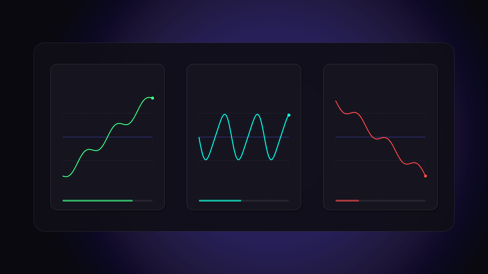
Abstract

This study tests how mean-reversion strategies perform in cryptocurrency markets. We formalized three classic mean-reversion signals into testable rules: Bollinger Band (z-score) reversion, the two-period RSI (RSI-2), and percentage distance from a moving average. Each was run across two assets (BTC/USDT, ETH/USDT), four timeframes (15m, 1h, 4h, 1d), and three market regimes (bull, sideways, bear). Of the planned grid, 78 backtests completed.

All strategies were run in their naked form, with no trend filter and no stop-loss, to isolate the raw edge of mean reversion before any risk overlay. The central finding: returns are driven mainly by market regime, not by which strategy you pick. Average returns ranged from +16.3% in bull regimes to -40.6% in bear regimes, a 57-point spread produced by identical logic. Two further findings: a high win rate does not mean a strategy is profitable, and faster timeframes systematically erode returns through transaction costs. We interpret these results against six decades of academic work on mean reversion and discuss what they mean for strategy design.

1. Theoretical Background: The Mean-Reversion Hypothesis

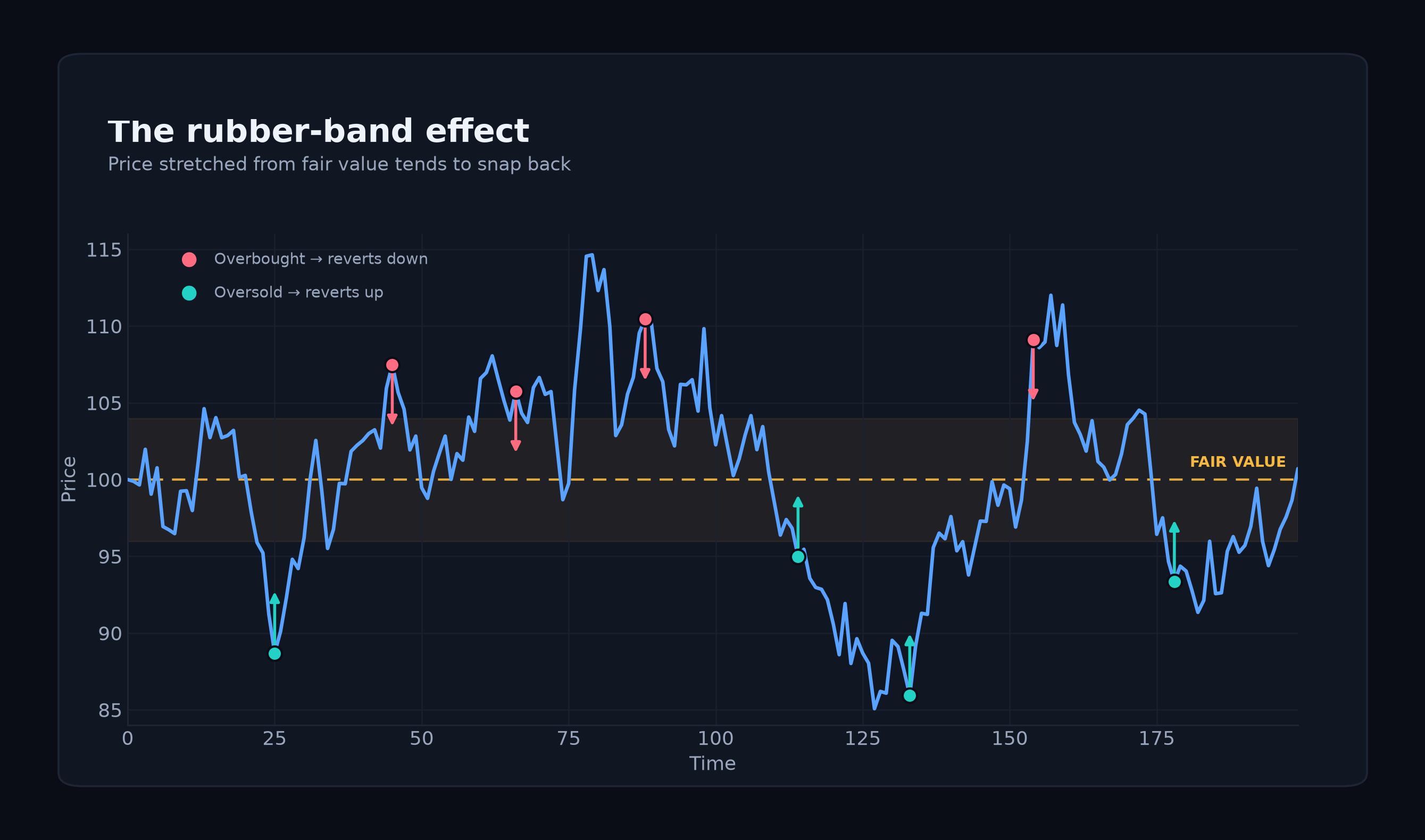
Most assets trade around a central value, a rough consensus of what they are worth. When a shift in sentiment pushes price away from that center, two forces are expected to pull it back: the initial sentiment fades, and opposing traders (bargain-hunters or profit-takers) step in. Together they push price back toward its center. That is the mean-reversion hypothesis.

Stated plainly: extreme moves away from a reference value tend to reverse. Unusually low prices are more likely to rise, and unusually high prices are more likely to fall. Not by any fixed mechanism, but because extreme states attract corrective reactions. The common intuition is an elastic band: the further you stretch it, the stronger the pull back.

1.1 How it differs from momentum (trend-following)

Mean reversion and momentum are opposite bets on price. Both work, but in different conditions.

Neither is better overall. Each works where the other fails. Section 4 tests this regime dependence directly.

2. Measurement Instruments: Three Displacement Metrics

Every mean-reversion strategy answers one question: how far has price moved from its normal range? They differ only in how they measure that gap. We use three.

2.1 Instrument 1: Bollinger Bands (the z-score)

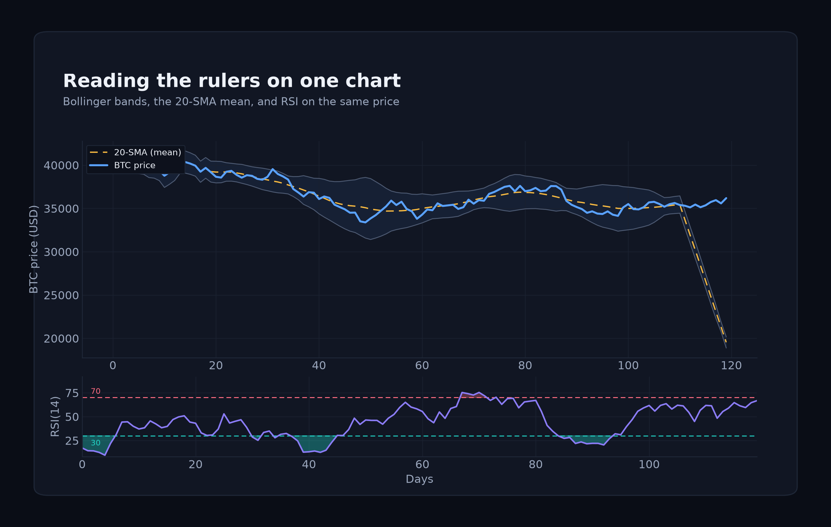
The z-score and Bollinger Bands measure the same thing. The z-score is the number; Bollinger Bands are that number drawn on the chart. The z-score is the distance of current price from its recent mean, measured in units of its recent standard deviation (its typical wobble):

z-score = (Current Price − Mean over N periods) ÷ Standard Deviation over N periods

• z = 0: price is exactly at the mean.

• z = +2: price is two standard deviations above the mean (unusually high).

• z = -2: price is two standard deviations below the mean (unusually low).

The ±2 threshold is where most mean-reversion strategies act. About 95% of past prices sit closer to the mean, so ±2 is genuinely rare territory. Bollinger Bands draw this on the chart:

• Middle band: the 20-period simple moving average (20-SMA).

• Upper band: 20-SMA + (k × standard deviation).

• Lower band: 20-SMA − (k × standard deviation).

The parameter k is just the z-score threshold. At the standard k = 2, a touch of the lower band means z = -2 and a touch of the upper band means z = +2. Because they are the same quantity, we call this "Bollinger Band reversion" throughout, while noting the band is the z-score.

2.2 Instrument 2: RSI(2), the short-horizon exhaustion gauge

RSI computed over a two-period lookback (RSI-2) was popularized by Connors as a short-horizon mean-reversion signal. Unlike the standard RSI(14), which tracks medium-term momentum, RSI-2 is very sensitive and can swing across its full range in two or three periods. It measures how exhausted the latest move is: below 10 means recent periods were almost all down (a stretched short-term drop), above 90 means the opposite. Many traders exit when it recovers above 70.

Read RSI-2 as an oversold-bounce gauge, not a trend indicator. It fires often, which is useful for higher-frequency testing, but it does not adjust for volatility. An asset with 8% daily swings hits RSI(2) below 10 as easily as one with 1% swings, even though that move is far less unusual.

2.3 Instrument 3: Percentage distance from a moving average

The simplest instrument measures how far price sits below its moving average, in percent:

Distance from MA (%) = (Current Price − Moving Average) ÷ Moving Average × 100

A reading of -5% means price is 5% below its 20-period moving average, and a fixed threshold (say -5%) sets the entry. The difference from Bollinger Bands is volatility handling: this metric uses a fixed threshold, so a -5% move counts the same whether it is ordinary or extreme for the asset. The z-score adjusts for recent volatility (a -5% move might be z = -3 on a quiet day but z = -0.8 on a wild one). In short, percentage distance is easier to read; the z-score is more robust for comparing across assets and regimes because it self-normalizes.

On CoinQuant, the percentage-distance-from-moving-average indicator is labelled "BIAS" in the interface.

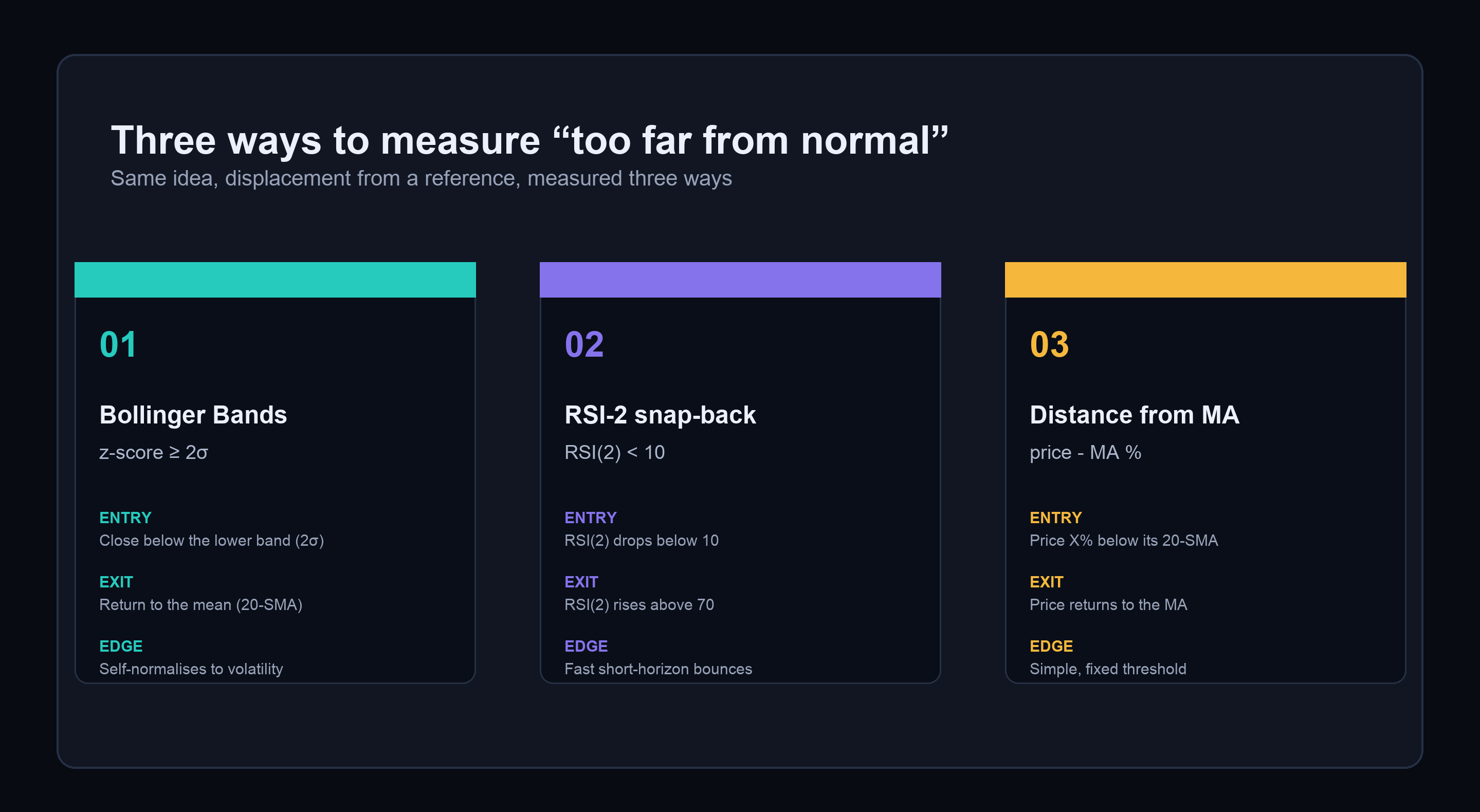
All three measure the same thing: how far price has moved from its normal range. The z-score adjusts for volatility, RSI-2 gauges short-term exhaustion, and percentage-distance states the gap in plain percent. Section 3 turns each into a concrete rule.

3. Strategy Specifications

These are baseline rules, written for clarity and reproducibility, not for maximum performance. Tune the parameters on a separate backtest before risking any capital.

3.1 Strategy A: Bollinger Band reversion (z-score entry)

Enter long when price closes below the lower Bollinger Band. Exit when it recovers to the middle band (the 20-SMA).

• Lookback: 20 periods

• k (z-threshold): 2.0 standard, or 2.5 for a stricter, more selective variant

• Entry: close crosses below the lower band, meaning price is more than 2 standard deviations below its 20-period mean

• Exit: close crosses above the middle band (back to the mean)

• Optional stop: close more than X% below the lower band

At k = 2, entries happen around the 5th percentile of recent price locations; at k = 2.5, around the 1st percentile: rarer, higher-conviction, but far fewer trades. The known failure mode is band-walking: in a strong trend, price can keep touching the lower band while it keeps falling. That is what motivates the regime filter in Section 4.

3.2 Strategy B: RSI-2 (Connors-style snap-back)

Enter long when the two-period RSI falls below 10 (extreme short-term oversold). Exit when RSI(2) recovers above 70.

• RSI period: 2

• Entry: RSI(2) closes below 10

• Exit: RSI(2) rises above 70 (or price closes above the 5-period SMA)

• Optional filter: only take entries when price is above its 200-period SMA, to avoid buying strong downtrends

RSI(14) is too slow for the short-term oversold conditions this strategy needs. RSI-2 is fast and suited to two-to-five-period bounce trades in ranging markets. The 200-SMA filter, part of Connors' original rules, keeps long entries out of strong bear markets.

3.3 Strategy C: Percentage distance from moving average

Enter long when price falls more than X% below its 20-period moving average. Exit when it returns to the average.

• Moving average: 20-period SMA

• Entry: price more than 5% below the 20-SMA (tune X), i.e. Distance from MA < -5%

• Exit: price closes at or above the 20-SMA (Distance from MA ≥ 0%)

Strategy C versus Strategy A:

In short: Strategy C is easier to read, Strategy A is more robust when volatility shifts.

4. Regime Dependence

Mean reversion is not condition-independent. It works in some regimes and fails in others, and getting the regime right matters more than tuning parameters.

4.1 A simple two-by-two model

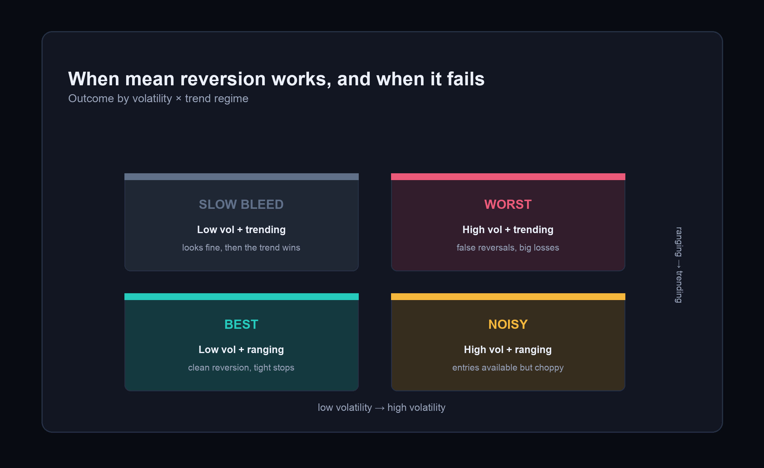
Strategy behavior sorts along two axes: trending vs. ranging, and high vs. low volatility.

The main risk is misreading direction. Price that has fallen to the lower Bollinger Band in a trending market is not oversold, it is riding a trend and likely to keep going. Running mean reversion inside a strong trend is like betting a heavy, fast-moving object will suddenly reverse.

4.2 A simple regime filter

Before applying any of the three strategies, check two things:

• Is price above or below its 200-period simple moving average?

• Is the Average Directional Index (ADX) above 25?

If both point to a strong trend, pause mean-reversion entries.

4.3 Worked example: the 2022 bear market

To make the regime effect concrete, we ran naive BB(20, k=2) reversion, long-only, exit at the midband, on BTC/USDT daily candles across 2022 (a bear year).

Result: -38.9% return, 33% win rate, 6 trades. The same figure reappears in the full grid (Section 7). The same run on ETH over the same window returned -39.3% with a 57% win rate.

The reason is simple. 2022 was a trending bear market, so each touch of the lower band was not a bargain but another step down. The elastic-band idea breaks when the reference level itself keeps drifting one way. The same rules over the 2023–2024 ranging-to-recovering market looked very different.

Before running any mean-reversion strategy, confirm the market is not trending. The 2022 BTC run also shows a statistical caveat: a 33% win rate over just 6 trades has almost no statistical power and should not be over-read. Always test across multiple regimes and larger trade counts.

5. Review of the Academic Literature

The seven most influential studies are summarized in the table below, each paired with a testable hypothesis for crypto on CoinQuant.

6. Methodology: Implementation on CoinQuant

No coding is required. This is the exact workflow used to generate every figure in this study, reproducible in minutes.

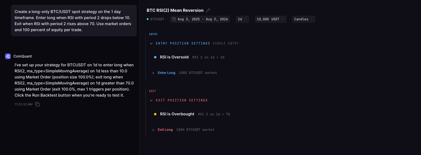
6.1 Step 1: Describe the strategy in plain language

In the CoinQuant strategy builder, you describe the strategy as a plain-language prompt and the platform compiles it into a testable strategy. No manual indicator setup. The exact prompts follow and can be pasted straight into CoinQuant (swap the asset, timeframe, and threshold as needed).

Prompt 1: Bollinger Band reversion (z-score entry)

Long-only BTCUSDT spot on the 1d timeframe on Binance. Bollinger Band mean reversion: enter long when the close crosses below the lower Bollinger Band (period 20, SimpleMovingAverage, k=2). Exit when the close crosses above the middle band (the 20-period SMA). Single position, market orders, 100% of equity per trade.

For the stricter variant, change k=2 to k=2.5 (wider bands, fewer entries).

Prompt 2: RSI-2 snap-back (Connors style)

Long-only BTCUSDT spot on the 1d timeframe on Binance. RSI-2 mean reversion (Connors style): enter long when RSI with period 2 drops below 10. Exit when RSI(2) rises above 70. Single position, market orders, 100% of equity per trade.

Prompt 3: Percentage distance from moving average

Long-only BTCUSDT spot on the 1d timeframe on Binance. Percent- distance-from-moving-average mean reversion: enter long when price is 5 percent below its 20-period SimpleMovingAverage of the close. Exit when price crosses back above the 20-period SMA. Single position, market orders, 100% of equity per trade.

The 5% threshold is for the daily timeframe. We scaled it down on faster charts (about 2.5% on 4h, 1.25% on 1h, 0.6% on 15m) to reflect the smaller spread around the mean at shorter horizons.

6.2 Step 2: Select the market

Each prompt sets the asset (we used BTC/USDT and ETH/USDT) and the timeframe (we tested 15m, 1h, 4h, 1d). Timeframe matters more than most people expect, as Section 7 shows.

6.3 Step 3: Run the backtest

CoinQuant runs each strategy against historical candles and returns the full metric set (total return, Sharpe, max drawdown, win rate, profit factor, trade count) net of realistic fees and slippage (see Section 7.1).

6.4 Step 4: Compare across regimes

The single most important rule: never judge a mean-reversion strategy on one backtest. We ran each strategy across separate bull, bear, and sideways windows, because the regime is the dominant driver of the outcome. This is the study's central finding, not a side note.

7. Results: 78 Backtests

We ran a pre-registered grid: 3 strategy variants × 2 assets (BTC, ETH) × 4 timeframes (15m, 1h, 4h, 1d) × 3 regimes (bull, sideways, bear). Of that grid, 78 backtests completed and are reported in full. Every rule was pure, naked mean reversion, no trend filter and no stop-loss, to measure the raw edge before any overlay.

The three instruments run as four configurations (Bollinger is tested at two band widths, since band width is its main tuning knob):

• Bollinger k = 2.0: classic Bollinger / z-score reversion (entry at the lower band, 2σ).

• Bollinger k = 2.5: stricter variant (wider bands, fewer, higher-conviction entries).

• RSI-2: Connors snap-back (entry at RSI(2) below 10, exit on recovery).

• Distance from MA (%): entry when price is unusually far below its 20-period moving average.

7.1 Experimental settings

Every result was produced under identical, transparent settings, with no cherry-picking.

The three windows were picked to be cleanly bull, bear, or sideways so the regime effect is unambiguous. They were identified from BTC price history and applied identically to both assets. Because real costs are charged on every fill, high-frequency strategies carry a visible cost burden. In one 15-minute Bollinger run, the strategy made 693 trades and paid over $2,300 in fees on a $10,000 account, the main reason fast-timeframe results fell apart (Section 7.4). A frictionless backtest would have hidden that entirely.

7.2 Main finding: regime is the dominant driver

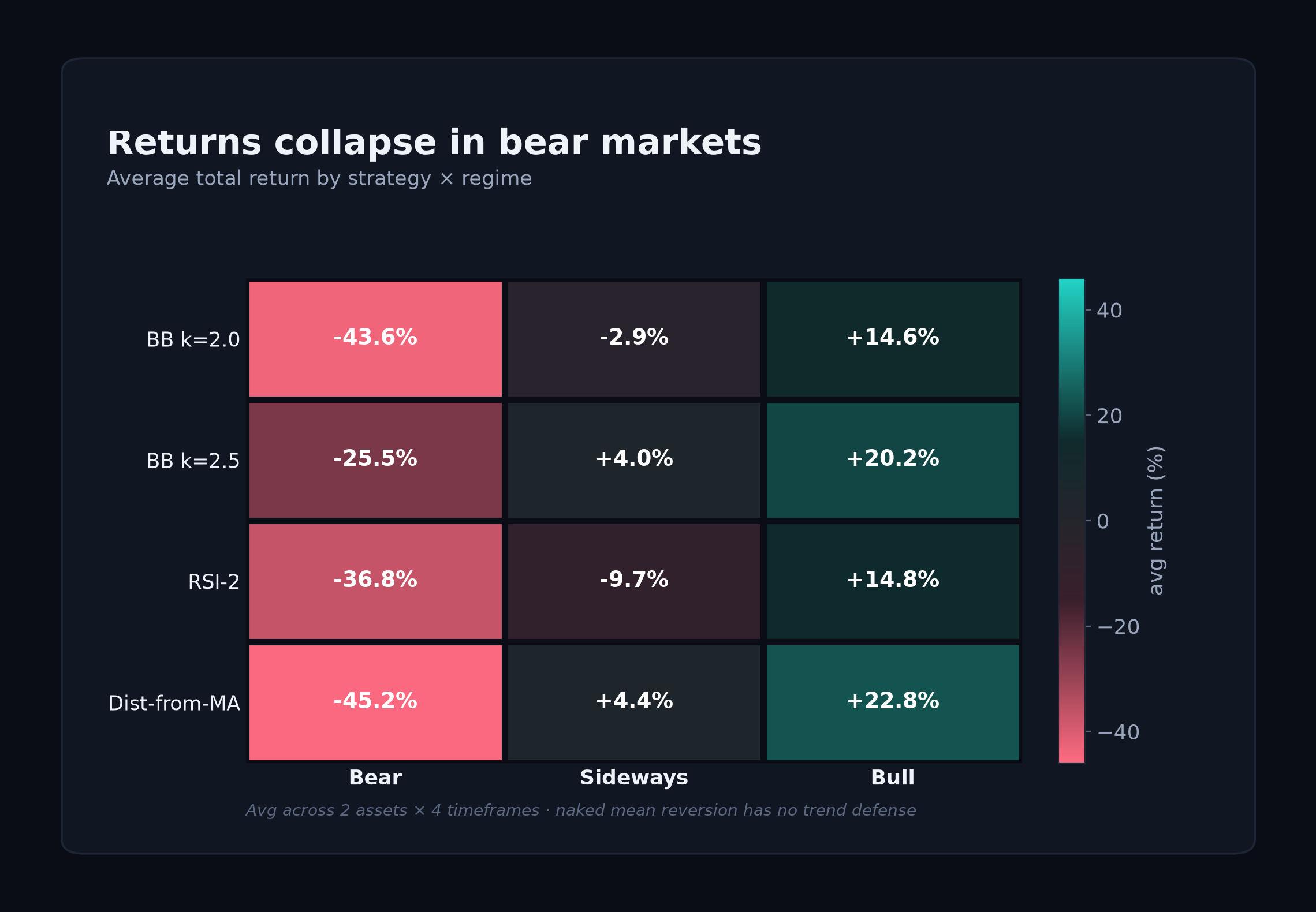
Average total return, across every strategy, asset, and timeframe, grouped only by regime:

This is the central result: a 57-point swing in average return, driven only by whether the market was trending down, ranging, or trending up. The logic never changed; only the regime did. Naked mean reversion has no sense of direction. In a bear market, every touch of the lower band looks like a bargain but is really another step down, so the strategy keeps buying a falling market. The elastic-band idea from Section 1 breaks once the reference level itself starts to drift.

7.3 The win-rate paradox

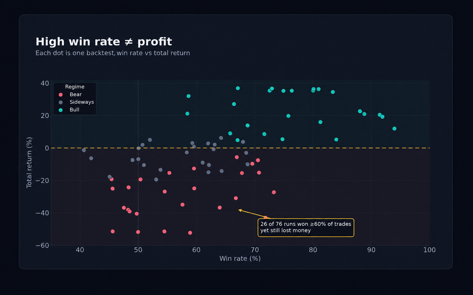
A result that matters for evaluating any strategy: 14 of the 78 backtests won 65% or more of their trades and still lost money. Examples:

• BB k=2.0, BTC, 1h, sideways: 68% win rate, -12.5% return.

• BB k=2.0, ETH, 1h, sideways: 68% win rate, -16.6% return.

• RSI-2, BTC, 1h, bear: 67% win rate, -21.9% return.

The reason is the payoff shape of mean reversion: it wins often but small (catching modest bounces) and loses rarely but big (when a supposed reversion turns into a trend and the position bleeds until the exit triggers well below entry). A 68% win rate looks great, but the 32% of losing trades outweighed the total gain from the 68% of winners. Loosen the bar from 65% to 60% and 26 of the 76 traded runs show the same pattern.

Win rate is one of the most tempting and least useful headline metrics in trading. Judge it alongside return, drawdown, and profit factor.

7.4 The transaction-cost effect of timeframe

Averaged across all conditions, returns generally improved as trading slowed down. The relationship is not perfectly monotonic (4h dipped just below 1h), but the endpoints are clear:

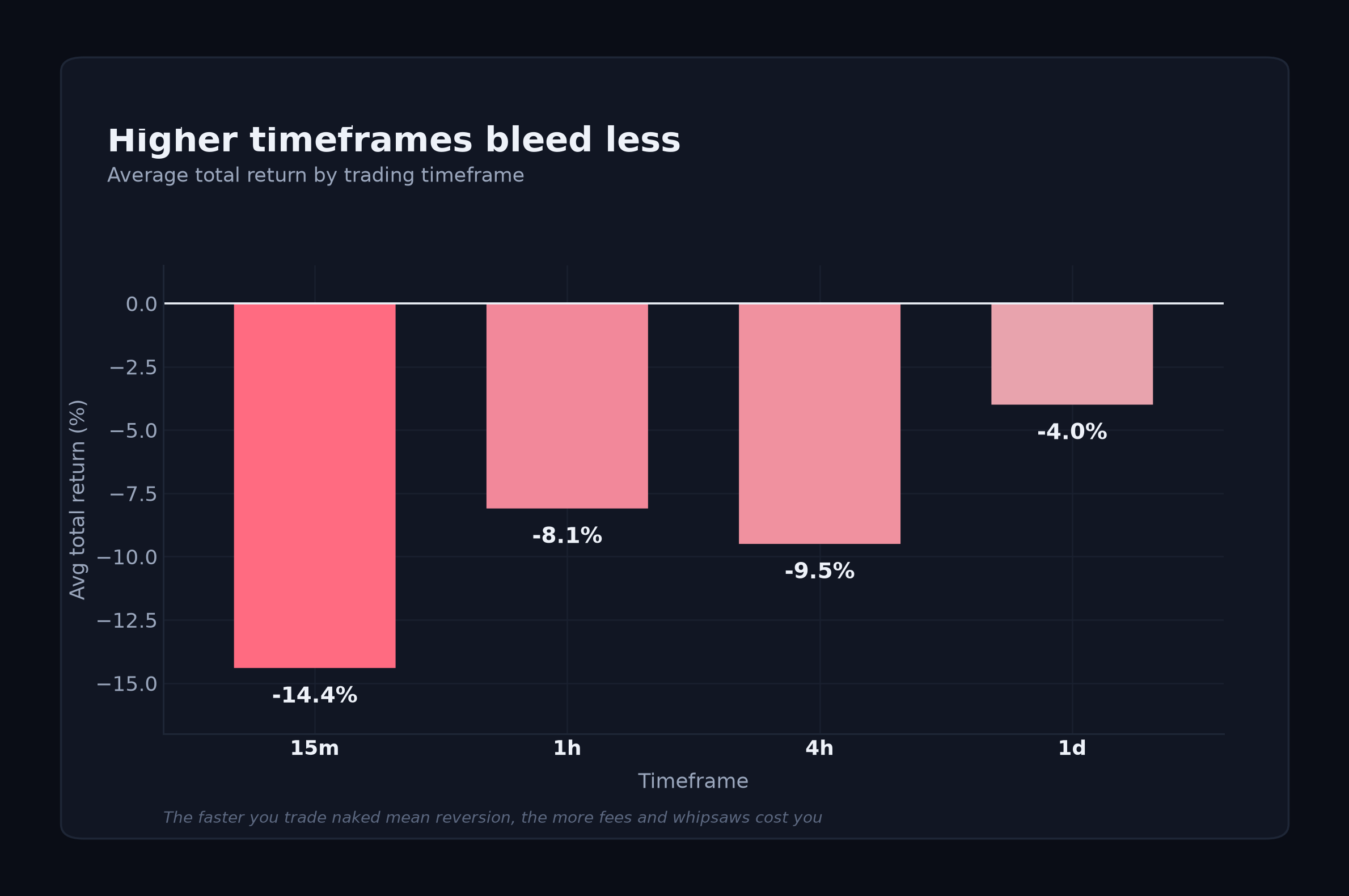
Faster trading of naked mean reversion adds two costs: fees (more trades mean more spread and commission) and whipsaws (intrabar noise triggers entries a daily candle would never see). As noted, one 15-minute Bollinger run made 693 trades and paid over $2,300 in fees on a $10,000 account, turning a positive gross edge into a net loss.

7.5 The strongest configuration

Of the four, percentage distance from moving average was the strongest on a risk-adjusted basis, with the best average Sharpe and the best average return. In good conditions it did exceptionally well:

• Distance-from-MA, BTC, 4h, bull: +30.1% return, Sharpe 2.52, 75% win rate.

• Distance-from-MA, BTC, 1d, bull: +25.6% return, Sharpe 2.57, 100% win rate (3 trades).

But the trade counts warrant caution: these Sharpe ratios often came from very few trades in the favorable regime. The same configuration averaged -45% in bear markets. It behaves like the others, strong in the right regime and damaging in the wrong one, differing only in degree.

7.6 Limitations and caveats

• Small samples. Several daily cells had only 2–6 trades. A 100% win rate over 3 trades means little; those cells are flagged, not hidden.

• Regimes labelled after the fact. Bull/bear/sideways windows were tagged in hindsight to isolate the regime effect. In live trading you don't know the regime in advance, which is exactly the problem the next study tackles.

• No trend filter or stops. Deliberate. We tested the naked edge so the added value of a protective overlay can be measured directly.

7.7 Full results: all 78 backtests

The complete 78-backtest ledger (three regime tables: bull, sideways, and bear, with per-cell return, Sharpe, max drawdown, win rate, trade count, and profit factor) is available to download below.

8. Discussion: Does the Literature Hold in Cryptocurrency?

Scorecard: how each academic claim held up against our CoinQuant backtests.

The remaining three claims (Lo & MacKinlay lead–lag, Jegadeesh cross-sectional reversal, Balvers et al. multi-year half-life) need multi-coin or longer-horizon designs beyond this grid and are left to later work.

8.1 Conclusion

The academic case for mean reversion survives contact with crypto data, with one big qualification: the edge is entirely conditional on market regime. Naked mean reversion is not a complete strategy but half of one. It spots when price is displaced, but says nothing about whether that displacement will reverse or continue. The missing piece is a trend filter.

Forthcoming in This Series

Next study: Adding a Trend Filter to Mean Reversion. Can the Bear-Market Bleed Be Eliminated? This study showed that naked mean reversion loses about 40% in bear markets by repeatedly buying a falling market. The next article adds a trend filter to the same strategies and re-runs the full 78-cell grid (same assets, timeframes, and regimes) to see whether one rule can turn the -41% bear outcome into a survivable one without giving up the +16% bull upside. We test several definitions of an adverse trend and report the full before/after on CoinQuant.

Test a mean-reversion strategy free on CoinQuant