Bitcoin Trading Strategy: 5 Approaches Backtested Over 7 Years

Most bitcoin trading strategies look good on paper. Fewer hold up when you add real fees, real data, and enough time for the market to surprise you. We tested five strategies on Binance BTCUSDT using CoinQuant's AI trading platform, pulling institutional-grade price data from Kaiko with 0.1% fees baked in on every trade. Here is what actually worked.

The strategies range from short-term mean reversion on 1-hour candles to multi-year trend-following systems. Some surprised us. One strategy returned over 770% across ten years. Another looked promising on a short window but faded when tested across a longer time horizon. The data tells the story.

This article explains how each strategy works, shows the backtest results, and gives you the exact steps to replicate these tests yourself on CoinQuant, no coding required.

How We Tested These Strategies

CoinQuant is a no-code AI trading platform that lets you configure, backtest, and deploy strategies without Python or Pine Script. For each test, we used:

• Exchange: Binance BTCUSDT (spot or perpetual)

• Data provider: Kaiko (institutional-grade tick data)

• Fees: 0.1% maker and 0.1% taker included on every trade

• No look-ahead bias: each signal is generated only on closed candles

Strategy 1: RSI Oversold/Overbought (Daily)

The RSI (Relative Strength Index) strategy is one of the most common bitcoin trading approaches. The logic is simple: buy when the market is oversold, sell when it is overbought. It is intuitive, easy to implement, and a reasonable baseline to measure everything else against.

Setup: Buy when RSI(14) crosses below 30. Sell when RSI(14) crosses above 70. Tested on daily candles.

What works: The strategy captures sharp recoveries after oversold conditions. On daily timeframes, signals are less frequent, which means fewer false positives and cleaner entries.

Common mistake: Running RSI mean reversion without a trend filter. RSI below 30 in a sustained downtrend can stay below 30 for weeks, generating a string of losing entries. Strategy 2 addresses this directly.

Strategy 2: RSI + SMA(200) Trend Filter (Daily)

This variant adds one rule to Strategy 1: only take the buy signal if price is above the 200-period simple moving average. If price is below SMA(200), the market is in a macro downtrend, and the trade is skipped entirely.

Setup: Buy when RSI(14) < 30 AND price is above SMA(200). Sell when RSI(14) > 70. Tested on daily candles.

The return is slightly lower than Strategy 1, but the SMA(200) filter is doing its job: keeping you out of trades during prolonged downtrends. Over a longer test period with multiple bear markets, this filter is likely to produce a bigger performance gap in its favor. Fewer trades, better quality.

Strategy 3: Bollinger Band Mean Reversion (12-Hour)

Bollinger Bands measure volatility by placing bands two standard deviations above and below a moving average. When price drops below the lower band, it signals an extreme move that statistically tends to revert. This strategy captures those bounces before the price recovers to the mean.

Setup: Buy when close drops below the lower Bollinger Band (20-period, 2 standard deviations). Sell when close rises above the middle band (the 20-period SMA).

Timeframe: 12-hour candles. More signals than daily, still filtered enough to avoid the noise of shorter timeframes.

The Sharpe ratio of 0.57 is better than both RSI strategies, meaning the returns are more consistent relative to the risk taken. The 12-hour timeframe strikes a useful balance: active enough to catch moves that daily candles miss, slow enough to avoid overtrading on noise.

Strategy 4: Bollinger Band Mean Reversion (1-Hour, 10 Years)

Same mean-reversion logic as Strategy 3, but on 1-hour candles with slightly tighter bands, tested across ten full years of BTC price history. This is the longest window in this article, covering multiple complete market cycles from below $1,000 to above $70,000 and back.

Setup: Buy when close drops below the lower Bollinger Band (10-period, 2 standard deviations). Sell when close rises above the middle band.

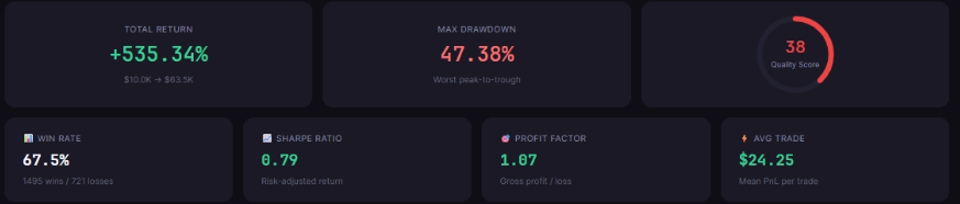
A Sharpe ratio of 0.79 over ten years of BTC is strong for a mean-reversion system. The 1-hour timeframe generates more trades than daily, which gives the statistical edge more chances to compound over time. The ten-year window gives this result far more credibility than the shorter tests above.

Strategy 5: Donchian Channel Breakout with Volume Confirmation (1-Hour)

Donchian Channels track the highest high and lowest low over a set number of periods. A breakout above the upper channel, confirmed by above-average volume, signals a potential trending move with real market participation behind it. Unlike the four strategies above, this one is trend-following rather than mean-reverting.

Setup: Buy when close breaks above the DC(20) upper band AND volume is above the 20-period volume SMA. Exit when close breaks below the DC(10) lower band.

The top performer in this test set. A 773.6% return over ten years with a Sharpe ratio of 0.79 means the gains were both large and consistent relative to the risk taken. The volume filter is the key differentiator: it eliminates false breakouts that occur on thin volume, keeping the strategy focused on high-conviction moves where real buyers are driving price.

Side-by-Side Comparison

What This Means for Your Bitcoin Strategy

Three patterns stand out from this data.

First, longer test windows reveal more. Strategies 4 and 5, tested over ten years, look dramatically different from the two-year snapshots. Short backtests can overfit to a single market phase, whether that is a bull run, a crash, or a sideways grind. Always test across multiple market cycles if the data is available. Two years of BTC data includes, at most, one full cycle.

Second, Sharpe ratio matters as much as raw return. Strategies 1 and 2 show 25-30% returns but a Sharpe of 0.50, meaning the equity curve was volatile. Strategies 4 and 5 delivered far higher returns with a Sharpe of 0.79, which translates to smoother compounding and less psychological pressure when managing live positions.

Third, trend-following outperformed mean reversion over BTC's full history. The Donchian breakout strategy beat every mean-reversion approach in this test. Bitcoin has spent most of its history in extended uptrends with occasional sharp drawdowns. That structure favors breakout and momentum systems over pure reversion plays.

What not to do: optimize a strategy on the same data you use to evaluate it. That produces numbers that look compelling in backtests and fail in live markets. CoinQuant's backtest engine enforces clean data separation to protect against overfitting.

How to Run These Backtests Yourself

You can replicate all five strategies on CoinQuant with no coding required. Here is the process, step by step:

1. Sign up at CoinQuant and connect your Binance account, or activate paper trading mode to test without real funds.

2. Open the Strategy Builder and select BTCUSDT as the trading pair.

3. Choose your timeframe: Daily, 12-Hour, or 1-Hour, depending on which strategy you want to test.

4. Add your indicator from the indicator library: RSI, Bollinger Bands, or Donchian Channel.

5. Set your entry and exit conditions using the visual condition builder. No Python. No Pine Script.

6. Set fees to 0.1% for both maker and taker to match the test conditions in this article.

7. Click Backtest and set your date range. Use at least three years of data for results that mean something.

8. Review the results panel: total return, Sharpe ratio, max drawdown, and trade count.

No Python. No Pine Script. No spreadsheets. The entire setup takes under five minutes per strategy. Run your own numbers, adjust the parameters, and find what works for your risk tolerance.
Find your best BTC strategy free